Animal locomotion is a complicate problem for the zoologist, starting from the mechanics of muscles and bones, but linked to physiology, reproduction, food consumption, ecological adaptation, animal metabolism, evolutionary pressure, and many other things that defy the naïve imagination of a physicist. It is therefore tempting to build ever more complex biomechanical models, with improved numerical methods and modelling techniques for animal locomotion, characterised by the interactions of fluids, substrates, and structures [ see e.g., the recent paper by Allen et al., Science Adv. 7, eabe2778 (2021) ].
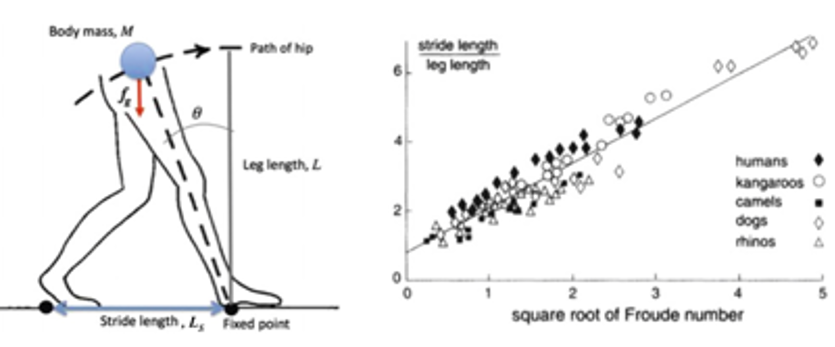
Notably, however, the kinematics of the simple pendulum, familiar to any first-year student of physics, has some impact on the behaviour of walking animals. Indeed, we can imagine a moving leg L attached to a body of mass M, akin to an inverted pendulum when it swings about a fixed point, identified by the point of impact of the foot (see enclosed figure, left). As the animal walks, the fixed point moves. However, if the walking frequency and the stride length are both taken as constant, we can assume that the fixed point is simply translated, and the alternate oscillations of the two legs are identical. With a bit of a leap of faith, the same relationship could be applied also to quadrupeds, by assuming that animals with four legs may coarsely be described as the sum of two animals with two legs, and a doubled mass (plus some phase relation coupling the fore and hind limbs).
By taking the most candid approach, let us imagine to have just some basic scientific notions, without knowing anything about mathematical physics. By looking at the pendulum bound to the string and constantly attracted downwards, we might suspect that gravity g must implied someway in its behaviour; furthermore, we could think it obvious that also the mass m of the ball; and the length L of the string, could also play a role. Therefore, we could invent a simple equation to describe the frequency v of the pendulum. In the ventures of dimensional analysis, we would write something like: v~magbLc. Then, we should just write the corresponding dimensional equation, considering that frequency has dimensions of [1/time], gravity is a [force]/[mass], and length is just… length. Therefore, [T–1]=[M]a[LT–2]b[L]c. By equating the respective exponents of T, M, L, we get easily a=0, b= –c=1/2, that is v~(g/L)1/2. This is just the classic equation of the pendulum, apart from numerical constants, showing that, contrary to the naïve assumption, the mass does not play a role in determining the frequency.
Biologists rarely believe in mathematics, and they prefer to collect hundreds of field data in the African savannah for animals of all sizes, from a rat to a giraffe [Alexander & Jayes, J. Zool. Lond. 201,135 (1983)]. Surprisingly (but only for them), they find that the walking frequency is a function only of the leg length L, and has nothing to do with the animal’s mass. Check out your inverted pendulum! However, this is not meant to dismiss the need for experimental observations. While quite powerful, the method of dimensional analysis relies on the expression of dimensional relations among quantities, and does not allow to determine the numerical values of the coefficients linking one variable to others. These must be obtained by experimental observations, or at least by informed theoretical models.
Another objection to the method of dimensional analysis is that, seemingly arbitrarily, we chose a power-law for the dependence of one variable (walking frequency) on the fundamental quantities (mass, length, time). Why we did not take, e.g., a logarithm, or a trigonometric, or a more complex function? The simplest way to understand it, is that a physical variable must not depend on the units in which it is measured. If we take the ratio between the values of the same physical variable for two samples, for example the masses of a horse and a mouse, this number must not change if we use kilograms or pounds as units. Such an independence is possible only if the defining equation in terms of the fundamental quantities has the power-law form.
Last but not least objection, with this method we can only determine the three exponents for mass, length and time. What if our problem has more than three variables? In reality, the harmonic development of the pendulum works for a walking animal only if the amplitude of oscillation, or “stride length” Ls, is small compared to L. But for an animal walking the inverted pendulum cannot be simply harmonic, since Ls is most often comparable to L, therefore it must enter in the determination of the frequency: we now have four variables to be determined with just three equations. To make things yet more complicated, we may want to compare animals walking or running at different speeds. What if in our problem of walking frequency, also the velocity u could be involved? The new relation should look like v~magbLcudLse, and we need five equations now. The corresponding dimensional equation is in this case: [T–1]=[M]a[LT–2]b[L]c[LT–1]d[L]e, with five exponents to be determined.
One way around this problem is that of reducing the number of variables, by empirically grouping them into non-dimensional numbers, a technique much used in engineering under the name of “Buckingham’s π-theorem”. In our animal walking problem, one obvious non-dimensional ratio would be Ls/L, let’s call this number P1. To construct a second ratio, one may think of the energies involved in our idealisation of a walk: there is the kinetic energy mu2/2 of the body translating horizontally with velocity u, and the potential energy mgL of the gravitational field to keep the body at a height L above the ground. Their ratio is obviously dimensionless, and may be another measure of comparison between animals of different weight and correspondingly different velocities. Therefore, we may write P2=u2/gL (forgetting about the numerical constants that give just a relative shift of the values). This parameter is again well-known in engineering, and is called the Froude number. The new equation for the walking frequency, including the arbitrary function of the two non-dimensional parameters, should be written as v~magbLc·f(P1,P2) and the corresponding dimensional equation is
[T–1]=[M]a[LT–2]b[L]c·P1·P2.
That is, we are back to the inverted pendulum of the simplest case, with the only difference that the numerical values of the dimensional relationship will change, as P1 and P2 change.
Well, it looks like we have added a lot of complication, not to gain much in this game. But we now have the two dimensionless variables that must mean something: the unknown function f(P1,P2)= = P1m ·P2n contains the idea that the qualitative behaviour of the walking frequency is unchanged if we look at animals having a similar ratio P1m /P2n . This is where we can learn something more than just the banal, inverse-square-root dependence of frequency versus length. The figure on the right [taken from R. Alexander, Math. Gaz. 80, 262 (1996)] plots the experimentally observed values of P1 vs. (P2)1/2, for a large variety of living animals. The fact that all the points for different animals, with different sizes and mass, living with different habits in largely different environments, either walking or running at different speeds, are instead nicely clustered along one same straight line, leads to deduce that the ratio of the two dimensionless parameters P1 and P2 must indeed provide a rather “universal” representation of the similarity of their walking characteristics.
To appreciate the instructive contents of this plot, notice for example the dependence of the Froude number on the inverse of g. When looking at astronauts walking on the Moon, we saw them moving in cumbersome, ‘floating’ steps, to the point that after some time they started making long jumps at a funnily low speed. In fact, since the gravity acceleration on the Moon is just 1.62 m s-2 compared to 9.81 m s-2 on the Earth, the P2 corresponding to a same walking speed increases by a factor of 5.6: to stay on the straight line in the plot, the value of P1 must therefore change to about 3, i.e., for an astronaut with a leg 1 m long, the walking stride becomes 3 m… Clearly, they need to make long jumps! The alternative to conserve a more normal walking length, would be to reduce the speed to less than 1 m/s: that would look like a slow-motion film.
Even more interestingly, the plot of P1 vs. (P2)1/2, also allows to formulate predictions for animals that are not being measured in this experiment, by using the same straight line as a guide. Maybe, also for extinct animal species: we actually dispose of fossil bones to determine L, and tracks of fossilised footprints to determine Ls. Then, how about dinosaurs? In the above cited paper, Alexander deduced walking speeds ranging from 1 m/s for the Brontosaurus (m ≃ 30 tons), to about 2 m/s for the Tyrannosaurus (m ≃ 5 tons), up to 12 m/s for the lightest, two-legged dinosaurs. I tried to estimate the speed of the scary Velociraptor from S. Spielberg’s Jurassic Park movie, by looking at their footprints and bones found in Arizona, which give Ls ~ 2.5 m and L = 0.75 m. Thus, we have P1= 3.3. Once situated on the straight line in the plot, this suggest a Froude number P2 ≃ 5.8, from which a velocity of about 7 m/s is obtained. That is about 25 km/h, a running speed faster than a mile-runner olympic champion, and definitely fast enough to catch the movie’s actors.
Therefore, large animals walk slowly, and the larger they are the less likely is they could actually “run”. There is increasing agreement that the classic claims about large dinosaurs being capable of running at blazing speeds, while being popularly attractive, are void of scientific support. Surely, there must be also key biomechanical constraints implicated, as far as joints, bone size, muscles and tendons, that must be adapted to each animal condition. For example, from another simple scaling principle we know that muscle force scales as the cross section of the muscle, therefore as the body mass to the power 2/3, while muscle weight obviously scales with power 1 of the mass. Hence, large animals must use their muscles largely to support their own weight in an isometric effort, and proportionally less is left to develop mechanically useable force, in comparison to more slender animals. Eventually, the simple scaling/dimensional model I outlined above appears to capture, and with minimal effort, much of the conclusions reached by richer and more complex studies, such as the Science paper cited in the beginning of today’s story. As ominous and scary as the T-Rex could appear, while watching that fantastic Jurassic movie I had instinctively considered the fast-runners Velociraptors to be way scarier than the big guy. Maybe, we human apes still carry deep in our mind an ancestral memory of our early days in the forests, when stealth and fast runners should have been more dangerous than slow and noisy behemots!