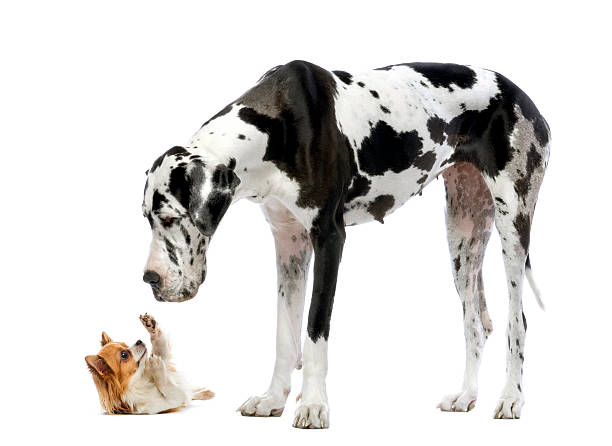
By looking around the natural environment, it is evident that both plants and animals of similar species vary in their size quite a lot more than us humans, notably as a function of certain genetic characters. A chihuahua is much a smaller dog than a Saint-Bernard, which however is as well a dog: the couple could in principle have a baby-dog, although the result might be quite weird. Moreover, sizes can vary as a function of environmental characters, for example, the amount and quality of food during the early development phases. However, in species taxonomy size is not always considered as an important factor, since it is deemed not central to determine the ancestry and relationships among species. Indeed, size can be adjusted according to natural selection, if some extreme conditions would favour a race of giant, or of dwarfs. Instead, a same body shape, albeit with quite extreme variations in size, is often an indication of a common ancestry. For example, whales and dolphins appear as two outstanding representatives of a same evolutionary design, although varying by factors of about 60 in size and about 2,000 in mass.
Nevertheless, extreme variations in size can have interesting consequences, as Jonathan Swift’s hero Gulliver discovered during his Travels into the Several Remote Nations of the World. Being both a surgeon and captain (but definitely not a physicist) mr. Gulliver, besides marvelling at the unusual size variation of the inhabitants of those fabulous countries, could have attempted a definitely more systematic study of functional variations as a function of the variation in animal body size. In Lilliput humans grow only to six inches, whereas in Brobdingnag they grow to 144 feet and higher. Swift probably chose those sizes because they were a handy factor of twelve, and no doubt this convenience made it easier for him to do the maths, having worked out that the Lilliputian foot corresponds to the Gulliverian inch while the Gulliverian foot is merely a Brobdingnagian inch. Swift, a British citizen of the 18th century, had no doubt spent most of his life doing conversions of twelves because of the peculiar English systems for measuring length and money (a pence was 12 to the shilling, and 240 to the pound).
Both Gulliver and Swift could have fared better by using the method of scaling analysis. Scaling analysis is not concerned with units, it looks for relationships that hold besides the particular numerical values. Let us compare two cubes, the one with side of 2 units and the other with side of 4 units. The surface of each face is 22= 4 for the first cube, and 42= 16 for the second one; their volumes are 23= 8 and 43= 64, respectively. However, the ratio of their surfaces is 4, in any unit of length we wish to measure it, and the ratio of their volumes is 8, in any unit as well. The size of the surfaces of the cubes is proportional to the square of their side lengths, and the size of their volumes is proportional to the cube of their sides. Also, scaling relations work independently on the shape of the object: if we consider the same quantities for two spheres, with radius 2 and 4 in whatever units, we would find the same relations. The example may look somewhat banal: if animals were to follow such a perfect scaling we could get, for example, the length of the intestines, or the amount of blood circulating in the veins of any dog, by scaling principles. To get such figures, we should firstly measure the length L of the intestines and the volume of blood V in one dog of a given size; then, by taking the ratio λ between, e.g., their nose-to-tail length, the size of the intestines of any other dog could be obtained by multiplying L by λ, or the blood volume by multiplying V by λ3. As weird as it may seem, such a method works more often than one could think. If you surmise that this is just a toy idea, and that you have better things to occupy your time on a Sunday, you would be surprised to learn that allometric scaling is routinely used to transform pharmacokinetics data from nonclinical studies in one or more animal species, to predict human drug exposure for a range of drug doses. This is a rapid method that can inform dosing decisions, or determine whether it is worthwhile to progress a particular therapeutic compound. In addition to predicting human exposure from nonclinical studies, allometric scaling is also used when moving between species, as the nonclinical program develops, as well as to predict drug doses for pediatric populations, by using data from adults.
Already in 1883, the German physiologist Max Rubner had used allometric concepts when studying animal metabolism and the heat dissipated by animals with bodies of different sizes. D’Arcy Thompson introduced more formally the idea in his celebrated 1905 book On growth and form. The general relationship of allometry for a quantity Msupposed to change as a function of the size scaling of another quantity x, is M = αxβ, where α is called the scaling coefficient and β the scaling exponent (for β=1 the scaling relation is linear, and the allometry becomes a simple isometry.) Biologists have a tradition of plotting allometric or suspected-allometric relationships on log-log graphs, so that anything that falls within this pattern comes out as a straight line. Anomalies in a log-log plot mean that the organism falls outside the expected proportions for one characteristic, even when scaled proportional to another one. The eye in vertebrate animals, for example, scales with negative allometry, meaning that in general, the eye gets smaller relative to the body weight as the organism gets larger. The blue whale has an eye the size of a football that, while certainly big, it is only a tiny fraction of its total body weight; conversely, a small mouse’s eye is a relatively large fraction of its body weight. Eyes, apparently do not get much better by simply getting bigger, and it is not biologically useful to the animal to try to grow a bigger eye as it gets larger. At the other end of the spectrum, eye capabilities would deteriorate quickly if they were to retain scaling with body weight, when humans are shrunk down to the size of the Lilliputians. The Lilliputians would all have been blind, or at least have very grainy vision, with their eye’s crystalline going from about 10 mm to 10 microns in diameter. At the opposite, the Brobdingnagians would confront the very problems that elephants confront: how to keep one’s body from crushing their legs. Elephant’s bones however are not as thick as logarithmic scaling would lead to expect. For an elephant’s femur to support the same fraction of its body weight, it would have to use about 70% of its body mass in pure bone. Elephants obviously don’t do that, so how do they survive? Well… by changing their behavior: they are slow, ponderous animals with no natural predators, so they can afford to become larger, even without strengthening their bones, because they have no need to pounce, jump and sprint for survival, like small mammals.
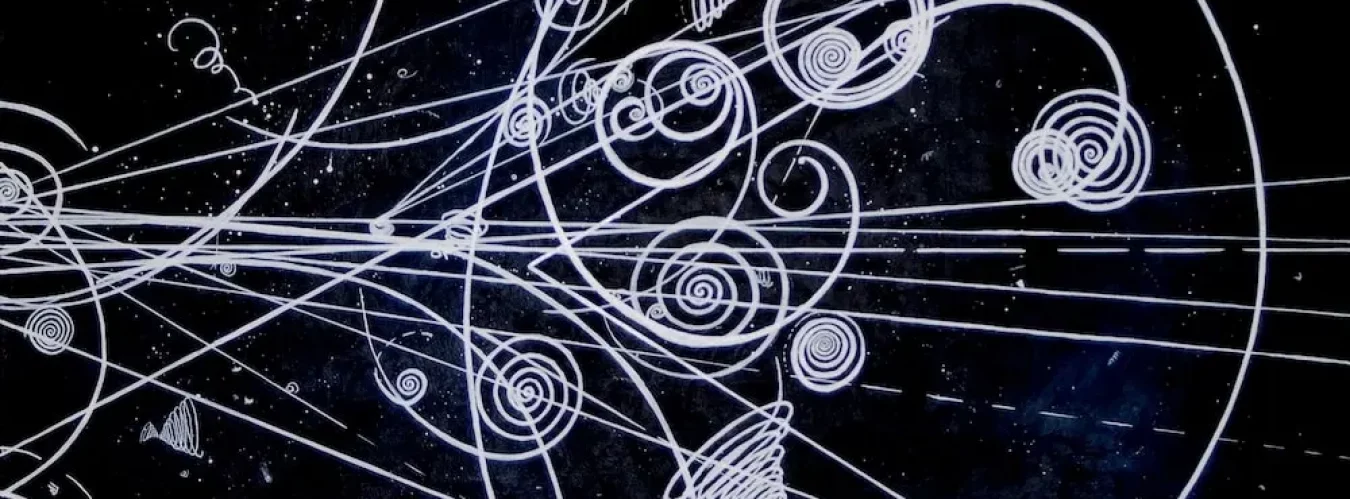
Scaling arguments play a central role in physics. In statistical physics, for example, scaling exponents naturally appear in the analysis of continuous phase transitions. Here, an observable of the system (an order parameter, such as magnetization in a crystal) quantifies properties of the system that change between different macroscopic states. At a critical value of a control parameter (e.g. temperature) the order parameter continuously grows from zero, indicating the emergence of a partially ordered state; near the phase transition point, the order parameter typically grows as a power law with the distance from the critical point. Critical exponents characterising continuous phase transitions often are universal: that is, their value is largely independent of the material properties but instead characterises the similarity of the underlying mechanisms, and the effective dimensionality of the underlying interactions across different systems. However, just like the eye of a whale does not grow to the size of a car, and elephant’s bones do not take up its whole body mass, scaling arguments must be used with caution also in physics. In any scaling law there is more than just the critical exponent, since its value alone is insufficient to quantitatively predict the value of the order parameters. A gentlemans’ polemic appeared a few months ago in Nature Physics serves as a good example.
A group of researchers from Bar-Ilan University (Israel) published a paper in which they unraveled universal features of signal propagation patterns in networks of dynamical elements, such as propagation of protein signals in the cell, epidemic spreading, ecological interactions and population dynamics, and similar [Hens et al., Nat. Phys. 15, 403 (2019)]. Sometime later, however, critics argued that under certain conditions a prefactor in a central expression of that paper was missing and that this prefactor would be important for predicting propagation times [see Peng et al. Nat. Phys. 16, 1082 (2020)]. In their reply, Hens and colleagues argued that common scaling analyses in statistical physics are made to deliberately neglect prefactors, and focus on scaling exponents, because just these reveal whether certain collective features are universal or not [Nat. Phys. 16, 1083 (2020)]. The conflict in the argument likely originates from a different interpretation of the notion of scaling, as well as a different meaning the respective authors assign to the mathematical symbol ~ . Hens is correct in claiming the universality of the exponents as a signature of universality, but also Peng is correct in requiring use of asymptotic scaling, to obtain absolute magnitudes of the claimed effects. In “ordinary” scaling we look at the slope of the ratio between two logarithms, the order parameter f(x) (e.g. magnetization) and the control parameter x (e.g., temperature). In asymptotic scaling we look for an expansion function g(x) that becomes asymptotically equal to f(x), as x approaches a critical point. Note that this is not simply a Taylor series, as asymptotic series often do not converge and exhibit intricate prefactors (see P.D. Miller, Applied Asymptotic Analysis, Amer. Math. Soc., NY 2006), the WKB approximation in quantum mechanics being an example of such analysis. As a simple example, let us consider the magnetization near the critical temperature, M=Aεβ, with ε=(T–Tc)/Tc. Finding the exponent β by scaling, as the limit for ε going to zero of the ratio lnM/lnε, points at the universality, but it is insufficient to quantitatively predict M, and constitutes only the first step of analysis. To obtain the value of M at any point where ε>0 we need a second step, namely to find the limit of lnM/lnεβ=A. The function εβ now contains a true predictive power.
At the turn of the century, Stephen Hawking stated that the twenty-first century will be the century of complexity, and he was certainly not thinking just of physics. Fully embracing the different aspects of scaling will be of great help in analysing and predicting phenomena across the multitude of complex systems that are at the frontiers of modern science.