In physics we have the custom of naming equations after the person who gave birth to them. However, the naming often translates to derivative products for which that person had not actually contributed, but is somewhat linked to it. See, e.g., the Boltzmann entropy equation, that was actually written down by Planck; or the Fermi energy, Fermi surface, Fermi temperature, etc, which Fermi never addressed in his works; or the Gauss’ laws (today known as the “first two Maxwell equations”), which were actually first discovered by Lagrange; or the Faraday tensor, which Faraday could never have used, since tensor calculus was introduced by Ricci only around 1890. Speaking of electromagnetism, the third of the so-called Maxwell equations (which were formulated by Oliver Heaviside, twenty years after Maxwell) was actually laid out in the experiments by Faraday and Henry, and is correctly labelled in some textbooks as the Maxwell-Faraday law… although it could be easily a Maxwell-Faraday-Henry law. Fact is, that the early formulations of both Faraday and Henry were unclear, and nobody in the mid-XIX century believed them to be true. It took Maxwell (and Heaviside) to write them in a proper mathematical form, to make them acceptable. And to be honest, a necessary corollary of the experimental laws was obtained by Emil Lenz, so that the entire law should rather be the “Maxwell-Faraday-Henry-Lenz law”. Luckily for the students, nobody calls it like that, and we have just a “third Maxwell’s equation”.
Faraday was unique in his thinking of magnetic phenomena. He visualized electric and magnetic lines of force as early as 1830 while working on his induction experiments. He wrote in his notes, “By magnetic curves I mean lines of magnetic forces which would be depicted by iron filings.” He opposed the idea that induction occurred by action at-a-distance, a vision that was prevailing in his time; instead, he held that induction should occur along curved lines of force because of the action transmitted by contiguous “particles”. Later, he envisaged that electricity and magnetism are transmitted through a medium that is the site of electric or magnetic “fields” (although he was very dubious about the concept of material ether). In 1831 he published his findings on electromagnetic induction, one year before Henry (who had discovered the phenomenon on qualitative grounds a few months earlier). But while Faraday found the proportionality between the electromotive force induced in a conductor and the (time or space) variation of the magnetic field, it took another three years for Emil Lenz to establish which is the direction of the induced current: as we know, it is such that the magnetic field generated by the current is opposed to the externally applied one. More on this to come.
In the paper he read before the Royal Society on 20 November 1845, Faraday announced the discovery he had made on 4 November, of “a new but very weak magnetic property of matter” whose observations “require magnetic apparatus of great power, and under perfect command”. To his own surprise, he had found that magnetism was not restricted to iron, nickel and cobalt, but was a property of nearly all “substances [which] appear to arrange themselves into two great divisions: the magnetic, and that which I have called the diamagnetic”. William Thomson soon provided mathematical rigor to this discovery, showing in May 1847 that the equations governing the behavior of (para)magnetic and diamagnetic substances under the influence of a magnet are the same but of opposite sign, thus illustrating Faraday’s conclusion that a diamagnetic substance is repelled by either polarity of a magnet. Notably, in his paper Thomson also first predicted the possibility of stable magnetic levitation of diamagnetic substances. Earlier experiments on liquid and solid materials were plagued by the confusion with optical phenomena, mainly propagated by Julius Plücker, and the complications added by crystallization of metal samples, which even led Fadaray to hypothesize a singular ‘magnecrystallic force’. It took the son of a poor Irish shoemaker, John Tyndall, to start seeing the microscopic structure of matter as critical to the mediation of force. With his careful experiments on crystals, cut, pressed and heated along different directions, Tyndall discovered the role of the direction of closest molecular packing in guiding the magnetic force, at a time in which atoms still were unobservable. Eventually, Faraday’s picture of field lines turned into Maxwell’s equations and Langevin’s model of diamagnetism. But Tyndall’s contribution, almost forgotten today, can only be retrieved in the definition of the magnetic susceptivity tensor.
As kids, we used to play with permanent magnets, for example pushing one end against the other and marvel at the repulsive force. Sometimes we could have tried to stack one magnet on top of another, trying to find an equilibrium position for which the magnet above would remain suspended over thin air. If you ever tried that, you may remember that it was a quite frustrating exercise, defeating even Monty Python’s noblest efforts “for putting things on top of other things”. The lack of an equilibrium configuration is not just a matter of your ability, it is strictly forbidden by a piece of mathematics dating from 1842, and known as the Earnshaw’s theorem. This actually follows easily from Maxwell’s equations (which poor Reverend Earnshaw couldn’t know, in his time). The energy of a permanent dipole M in a field B (both vectors) is U = –M·B. Since the (x,y,z) components of M are constant, the Laplacian of the energy is just ∇2U= –∇(M∇·B)=0 in free space. This means that there is no point of stability, hence your little magnet can never find an equilibrium position on top of the other magnet. However, with all of its might, Earnshaw’s theorem does not strictly apply to diamagnetic materials but only to ferromagnets. The induce diamagnetic field is not permanent, but adapts constantly to the changes in the external field, making magnetic levitation a possibility. This can be seen again by the previous equation: for an induced dipole it is M=kB, with k a constant, negative for diamagnetic or positive for a paramagnetic material. In this case the Laplacian of the energy is equal to ∇2U= –k∇(∇·B2), which is greater than or equal to zero. Hence, for diamagnetic materials some equilibrium configuration becomes possible, provided B is changing in time and/or space.
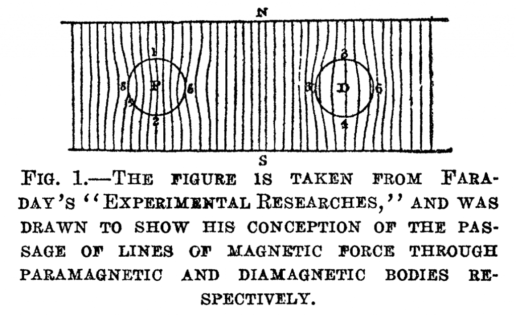
Although it says nothing about the magnitude of the field, Lenz’s experimental observation is enough to understand magnetic phenomena, once we have a quantum theory of the electrons in the solid state. Diamagnetism would be the natural response of any material, when its electrons are all paired in the quantized energy levels: the interaction between the external field has opposite results on each electron in a spin pair, their contributions cancel out, and the net induced field is zero. Only a weak magnetic component arises from the perturbation of the orbital momentum of the electrons, directed against the external field in agreement with Lenz’s law: diamagnetism is essentially related to the expulsion of magnetic field lines from inside the material, as Faraday had already understood in his drawings (see enclosed picture). As a result, the (very few) materials that display a somewhat stronger diamagnetism can truly levitate, for example a thin pyro-graphite leaflet deposited on a strong permanent magnet. A special case is that of superconductors, ideal diamagnets in which the magnetic field is completely expelled from the material, giving rise to the Meissner effect and to somewhat more spectacular levitation effects.
The word levitation obviously comes from the Latin levis, “lightweight”; however, its use goes back to XVII century England, where the verb “levitate” was created as opposite to “gravitate”, to indicate the ability of saints to rise in the air, and of witches to fly against their weight. The most famous eponym was Saint Joseph of Copertino, who had perfected the art to the point of flying backwards and upside-down. In modern times, levitation has gained interest in nanoscience, where levitation of nano- and micro-objects in high vacuum conditions can provide ideal isolation from the environment, while coupling the internal degrees of freedom (e.g., phonons, magnons, excitons) to controlled external degrees of freedom (translation, rotation). For example, the most precise commercial accelerometers are based on levitating systems, achieving sensitivities better than 10−11 g/√Hz. Today, levitation is achieved with a variety of electro-optical devices, such as the optical tweezers (see the recent review in Science by Gonzalez Ballestero et al.). However, compared to optical and electrical traps, magnetic trapping has the advantages that it can also work with nearly macroscopic objects, can avoid photon scattering that leads to decoherence, and photon absorption that leads to heating the sample, and can reach very low frequencies. The exotic discipline of quantum magnetomechanics explores different techniques to prepare and control quantum states of a mechanical oscillator using magnetic interactions (i.e., Lorentz force instead of radiation pressure), such as magnetically levitated objects coupled to, e.g., a superconducting circuit, superconducting qubits, or even spin qubits, for readout and control of the device. Quantum magnetic coupling can also provide cooling, to freeze the center of mass motion of the levitated system in its quantum ground state, even for objects as large as 1014 atoms.
Another (much simpler) way to keep an object steady about a point or a trajectory, is to impart it a fast angular rotation. Conservation of angular momentum will resist external perturbations, at least up to a certain point, and the object will maintain its kinematic conditions. From Euler’s equations, which relate the moments of inertia and rotation velocity to external torque, it can be easily proved that a rigid body is stable against small perturbations when rotating about the axes of largest or smallest moments, an effect exploited for example in the gyroscope of your cell phone. The same effect is used in the Levitron, a popular toy with a levitating spinning top made from permanent magnets, demonstrating that also rotation can simply beat Earnshaw’s theorem (you may try to build one at home using a large magnet from an old stereo speaker). But the more I dig into Albert Einstein’s works, the more interesting and unusual papers I discover, and here comes something about spinning charges and magnets. You are certainly in good company if you think that Einstein was a perfect theorist who never touched an experimental tool by his hands. However, he took part every now and then in some actual experiments, and in 1915 he signed a series of experimental papers as first author, together with Wander J. De Haas, on what is known today as the Einstein-De Haas effect (or EdH).
Einstein’s motivation in these works seems to go back to the problem of stability of the atom in Maxwell’s electromagnetism (but ignoring Bohr’s paper of 1913) and to the issue of zero-point motion (which I already treated in a previous letter). To prove Ampere’s hypothesis that magnetism has its microscopic origin in the circular motion of electric charges, Einstein and De Haas set up an experimental arrangement in which a tiny metallic cylinder was suspended inside a solenoid. The idea was that, upon changing the current in the solenoid, a corresponding change in the magnetization ΔM should occur. If the magnetic force is due to circulating charges inside the metal, angular momentum ΔL must be conserved, and the rodlet must start rotating with a constant λ=ΔL/ΔM. This is indeed was they observed, and in their second paper of 1915 Einstein and De Haas happily noted that the measured value of λ was in good agreement with Einstein’s previous theoretical prediction. However, electron spin was not yet discovered by that time, and they could consider only the orbital motion of the charges. As it later turned out, their measurement was wrong by a factor of (guess…?) exactly 2, since what they were actually measuring was the gyromagnetic ratio of the electron. However, this experiment and the ideas behind it went a long way; for example, it ushered in the whole family of magnetic resonance spectroscopies, and finds recently some quantum analog in molecular spintronics. In analogy to the classical EdH effect, magnetization reversal in a single-molecule magnet (such as, a phthalocyanine complexed with a metal ion) results in a rotation of the molecule, to satisfy conservation of angular momentum and energy; if the molecule is coupled to a nanomechanical resonator (for example, a carbon nanotube), this reversal can be detected as a quantized phonon mode in the resonator, in a quantum version of the EdH effect.